
Uncertainty in Supply Chain Optimization
- RobParkin
- Mar 8, 2019
- 6 min read
Uncertainty is typically not well handled in modern supply chain management systems. Most systems really only consider potential uncertainty in demand for an item. They ignore uncertainties on the vendor side like variations in their ability to supply and item quality. Even when they do look at uncertain in demand, they typically use a static safety stock measure to calculate how much inventory should be held back to prevent stockouts. In these cases a supply chain analyst must set a service level (i.e., the probability of meeting demand without a stockout) and this is used along with the mean and standard deviation of historical demand to determine how much inventory to reserve for unexpected events. There are several issues with this approach that can lead to very bad business outcomes for the company. Michel Baudin and Billy Hou have written articles that discuss the common issues.
A better approach would be to directly incorporate the uncertainty in both demand and the vendors ability to fulfill directly into a formal optimization model. In this way, the decisions made could directly utilize what is known about the risks on both sides of the equation. In this post, I will use a simple Bayesian model to one approach for how this might be done.
Our Supply Chain Optimization Problem
For simplicity let's assume that we have three suppliers from whom we can order our part. These suppliers have different prices, different quality items, and different maximum amounts they can ship to us within a certain timeframe. We know the prices and max order sizes, but the true yield distribution is unobserverable. Here, we include the unobservable parameters VENDOR_YIELD and VENDOR_YIELD_SD to simulate data, but we will assume we don't know them. VENDOR_YIELD is the mean yield of a given supplier while VENDOR_YIELD_SD is the standard deviation away from that mean. The standard deviation gives you a simple measure of the variability of the supply from that supplier.
In this case, the first supplier will be more expensive ($220) but will be more reliable (lower SD) and have the highest max order size. Vendor #2 is the least reliable and has the lowest ability to supply but is also significantly lower in cost. Vendor #3 is in the middle on every metric.
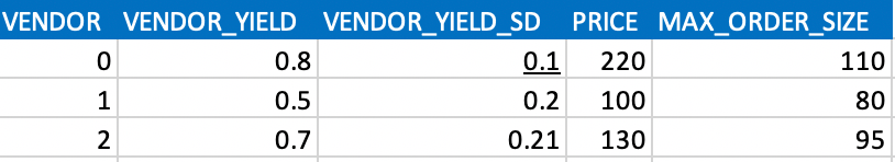
The yield represents the percentage of parts that pass our quality test and arrive on time. Due to different manufacturing techniques, the yield varies quite a bit, which is also reflected in the price. As we assume that we can't directly observe the true yield, we will have to estimate it from previous batches we ordered. Let's assume we have ordered a different number of times (N_OBS) from different vendors. For example, as vendor 2 (third list item) only opened up recently, we only ordered twice from there:
Let's create some data based on those inputs:
So this is the data we have available to try and estimate the true yield of every vendor.
Quick note on the generality of this problem:
Almost every retailer (like Amazon) has this problem of deciding how much to order given yield and holding cost. A similar problem also occurs in insurance where you need to sell contracts which have some risk of becoming claims. Or in online advertising where you need to decide how much to bid on clicks given a budget. Even if you don't work on these industries, the cost of any inefficiencies gets passed onto you, the customer.
The Dynamics of the Supply Chain
In order to assess how many parts we need, we first need to know how many final products we can sell. If we buy too few, we are leaving money on the table; if we buy too many, we will have to put them in storage which costs money (HOLDING_COST). Let's assume we can sell a product for $500 and it costs us $100 to stock the product in inventory.
Next, let's define our loss function which takes as inputs how many parts we have in stock, how many final customers want, at what price we bought the part, at what price we can sell the product, and what the holding costs are per product:

As you can see, if customer demand is 50, we maximize our profit if we have only 50 items in stock. Having fewer eats into our profits at a greater rate than ordering excess product because in this situation our margins are larger than the holding cost.
Next, we need our estimate of demand. As we have a long history of sales we have a pretty good idea of what the distribution looks like, but we will also assume that we don't know the true underlying parameters and only have access to the samples:

In response to demand, the loss-function behaves differently: with less demand than what we have in stock, we earn less (because we sell fewer final products but also have to pay holding costs). However, as demand exceeds the number of parts we have in stock, our profit stays flat because we can't sell more than what we have.
Estimating yield with a stochastic model
Let's build a model to estimate the yield of each part vendor:

Generate possible future scenarios
In order to perform do the optimization, we need an estimate of what the future might look like. As we are in a generative framework this is trivial: we just need to sample from the posterior predictive distribution of our model which generates new data based on our estimated posteriors.
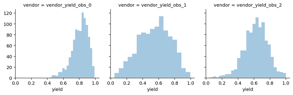
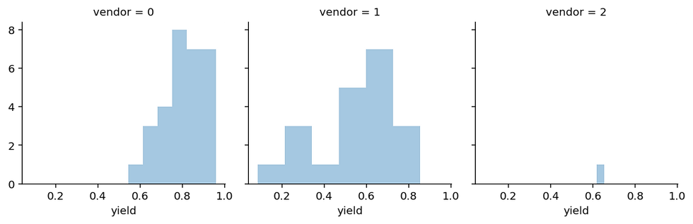
This plot shows, given the data and our model, what we can expect to observe. Note that these predictions take the uncertainty into account. For vendor 2, we have a lot of uncertainty because we only observed very few data points.
Given these estimates we can write a function that calculates the orders we place to each vendor, the yield we assume for each one, and what their prices are going to be.
So given these (randomly picked) order amounts to each vendor and some deterministic yield, we would receive 168 functioning parts at an effective price of $162.72 each.
Bayesian Decision Making
Now we have to actually do the optimization. First, we need to specify our objective function which will compute the total yield and effective price given a posterior predictive sample. Once we have that and our demand (also a sample from that distribution), we can compute our loss. As we have a distribution over possible scenarios, we compute the loss for each one and return the distribution.
Great, we have all our required functions. Now let's put things into an optimizer and see what happens.
Great, we did it! But is it actually any better than just assuming the means of the yield distributions for each vendor?
Evaluation
To build a more compelling case, we can compare the deterministic method (just using the means) with our stochastic approach and see which one generates more profit from the simulation.
Instead of samples from the posterior predictive, we can just pass a single sample (the mean) into our objective function. We can also just pass in the average expected demand (100). This way we can still use the above objective function, but the loop will only run once.
The results are certainly different. The stochastic model seems to dislike our high-cost but high-quality vendor. It also orders more in total (probably to account for the lower yield of the other two vendors). But which one is actually better in terms of our profit?
To answer that question, we will generate new data from our generative model and compute the profit in each new scenario given the order amounts from the two optimizations.

As you can see, the stochastic model has a profit of $340.78 and the deterministic model only yields $320.48.
Summary
Clearly adding information about the uncertainty in both demand and supply can improve the results from a supply chain optimization model. In fact there is a mathematical proof that shows this is always a better option. There are also intuitive reasons. Namely, we are not just optimizing over the most likely scenario, we are taking into account a large number of potential future scenarios. Also note that we were able to do the optimization using just samples (as opposed to integrating over the probability distributions). This gives us a lot of flexibility in that we can arbitrarily extend our models while still using the same uncertainty framework.


Comments