
Variational AutoEncoder
- RobParkin
- Oct 5, 2017
- 4 min read
Updated: Oct 1, 2020
The main motivation for this post was that I wanted to get more experience with both Variational Autoencoders (VAEs) using Tensorflow.
Autoencoders are an unsupervised learning technique in which we leverage neural networks for the task of representation learning. Specifically, we'll design a neural network architecture such that we impose a bottleneck in the network which forces a compressed knowledge representation of the original input. If the input features were each independent of one another, this compression and subsequent reconstruction would be a very difficult task. However, if some sort of structure exists in the data (ie. correlations between input features), this structure can be learned and consequently leveraged when forcing the input through the network's bottleneck. The key is that the encoding network will output a single value for every encoding dimension. The decoding network then attempts to recreate the original input based on those values.
The distinction for variational encoders is that try to describe observations in the latent space in probabilistic terms. Instead of having the encoder produce a single output for each attribute, it tries to estimate the probability distribution that best describes it.
By constructing our encoder model to output a range of possible values (a statistical distribution) from which we'll randomly sample to feed into our decoder model, we're essentially enforcing a continuous, smooth latent space representation. For any sampling of the latent distributions, we're expecting our decoder model to be able to accurately reconstruct the input. Thus, values which are nearby to one another in latent space should correspond with very similar reconstructions.
By sampling from the latent space, we can use the decoder network to form a generative model capable of creating new data similar to what was observed during training. Specifically, we'll sample from the prior distribution p(z) which we assumed follows a unit Gaussian distribution.
Let us first do the necessary imports, load the data (MNIST), and define some helper functions.
Initialize the network
We need to initialize the network weights. To do this we will follow Xavier and Yoshua's method (http://proceedings.mlr.press/v9/glorot10a/glorot10a.pdf)
Create the Autoencoder
Based on this, we define now a class "VariationalAutoencoder" with a sklearn-like interface that can be trained incrementally with mini-batches using partial_fit. The trained model can be used to reconstruct unseen input, to generate new samples, and to map inputs to the latent space.
In general, implementing a VAE in tensorflow is relatively straightforward (in particular since we do not need to code the gradient computation). A bit confusing is potentially that all the logic happens at initialization of the class (where the graph is generated), while the actual sklearn interface methods are very simple one-liners.
We can now define a simple function which trains the VAE using mini-batches:
Illustrating reconstruction quality
We can now train a VAE on MNIST by just specifying the network topology. We start with training a VAE with a 20-dimensional latent space.
Epoch: 0001 cost= 174.838499673
Epoch: 0006 cost= 109.187535234
Epoch: 0011 cost= 104.770604595
Epoch: 0016 cost= 102.271029413
Epoch: 0021 cost= 100.553602004
Epoch: 0026 cost= 99.354442014
Epoch: 0031 cost= 98.556810455
Epoch: 0036 cost= 97.884472906
Epoch: 0041 cost= 97.332377583
Epoch: 0046 cost= 96.849344371
Epoch: 0051 cost= 96.464298193
Epoch: 0056 cost= 96.070154086
Epoch: 0061 cost= 95.763397147
Epoch: 0066 cost= 95.485776894
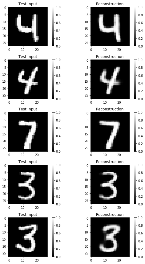
Epoch: 0071 cost= 95.238320451Based on this we can sample some test inputs and visualize how well the VAE can reconstruct those. In general the VAE does really well.
Illustrating latent space
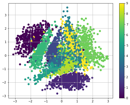
Next, we train a VAE with 2d latent space and illustrates how the encoder (the recognition network) encodes some of the labeled inputs (collapsing the Gaussian distribution in latent space to its mean). This gives us some insights into the structure of the learned manifold (latent space).
Epoch: 0001 cost= 191.034452792
Epoch: 0006 cost= 153.924423800
Epoch: 0011 cost= 148.399048934
Epoch: 0016 cost= 145.878458474
Epoch: 0021 cost= 144.328441190
Epoch: 0026 cost= 143.220495106
Epoch: 0031 cost= 142.397664823
Epoch: 0036 cost= 141.764116585
Epoch: 0041 cost= 141.174636827
Epoch: 0046 cost= 140.639492534
Epoch: 0051 cost= 140.267117532
Epoch: 0056 cost= 139.803164271
Epoch: 0061 cost= 139.496614824
Epoch: 0066 cost= 139.324203269
Epoch: 0071 cost= 139.021045699
Visualization of latent space
To understand the implications of a variational autoencoder model and how it differs from standard autoencoder architectures, it's useful to examine the latent space. This blog post introduces a great discussion on the topic, which I'll summarize in this section.
The main benefit of a variational autoencoder is that we're capable of learning smooth latent state representations of the input data. For standard autoencoders, we simply need to learn an encoding which allows us to reproduce the input. Focusing only on reconstruction loss does allow us to separate out the classes (in this case, MNIST digits) which should allow our decoder model the ability to reproduce the original handwritten digit, but there's an uneven distribution of data within the latent space. In other words, there are areas in latent space which don't represent any of our observed data.
On the flip side, if we only focus only on ensuring that the latent distribution is similar to the prior distribution (through our KL divergence loss term), we end up describing every observation using the same unit Gaussian, which we subsequently sample from to describe the latent dimensions visualized. This effectively treats every observation as having the same characteristics; in other words, we've failed to describe the original data.
However, when the two terms are optimized simultaneously, we're encouraged to describe the latent state for an observation with distributions close to the prior but deviating when necessary to describe salient features of the input.
An other way of getting insights into the latent space is to use the generator network to plot reconstructions at the positions in the latent space for which they have been generated:
The figure below visualizes the data generated by the decoder network of a variational autoencoder trained on the MNIST handwritten digits dataset. Here, we've sampled a grid of values from a two-dimensional Gaussian and displayed the output of our decoder network.
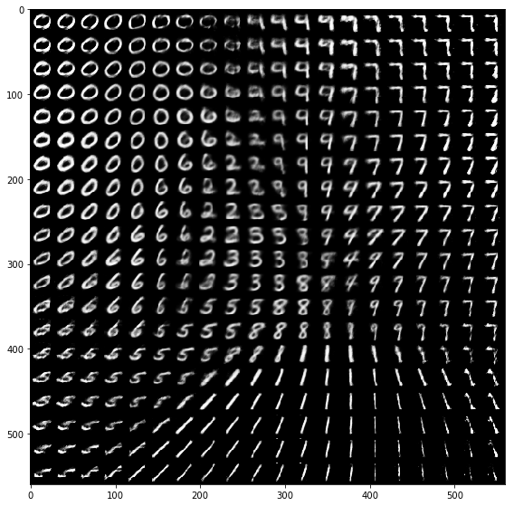
As you can see, the distinct digits each exist in different regions of the latent space and smoothly transform from one digit to another. This smooth transformation can be quite useful when you'd like to interpolate between two observations.


Comments